

Disclaimer:
The authors are solely responsible for the content of this report. Material included herein does not represent the opinion of the European Community, and the European Community is not responsible for any use that might be made of it.
Back to overview reports
The “cubage”-technique (“kubatuur” in Dutch) is a relatively simple technique to calculate the hydrodynamics in an estuary (Smets, 1996; Plancke et aL, 2011). It requires only topo-bathymetric data and water levels at different stations to calculate discharges and cross-sectional averaged flow velocities (see Figure 3) starting from the conservation of mass formula. In contrast to numerical process models, this technique does not require any flow resistance (“roughness”) coefficients to calibrate the model. Where the cubage technique uses mass conservation (which is an exact relationship) the error of the method is solely related to the error in water level and topo-bathymetric data. Hereafter some mathematical background on this technique is given.
The hydrodynamics in a river or estuary can be described in a one-dimensional way using following equations:
with:
Output parameters
The “cubage”-technique calculates discharges in time between every 2 consecutive cross-sections in the estuary. From this parameter following additional parameters can be derived:
Within the TIDE-project it was chosen to perform the cubage calculation for mean tidal conditions (only input data available for mean tidal conditions). In a first step the mean tidal parameters (HW, LW, time of rising and time of falling) were derived from measurements for the present situation for a station at the mouth, a station in the middle of the estuary, and a station at the upstream boundary of the estuary (see Table 3). Where the cubage technique requires a continuous time series of water levels, one period (or 2 periods for the Elbe and Humber) with several tidal cycles was chosen from the continuous measurements (see ‘selected tides’ Table 3) for which the low and high waters have the best agreement with the MHWL and MLWL values for the present situation for all 3 selected stations. For the Elbe and Humber 2 time periods were selected (one with low and one with high river discharge) because of the important differences in river discharge at the up-estuary boundary of these estuaries. From the selected time period, water level measurements for all tidal stations were selected as input for the cubage calculation (location of all tidal stations see Figure 9 (Scheldt), Figure 10 (Elbe), Figure 11 (Weser) and Figure 12 (Humber)) .
In a next step cross sections were defined perpendicular to the thalweg. The thalweg is defined as the longitudinal profile linking the deepest points of each cross section. The distance between two sections was chosen at about 500 m: this resolution was on the one hand sufficient to represent the topo-bathymetry, while on the other hand the number of cross section remained acceptable. These cross sections were exported in a MIKE11-format. Subsequently the different cross sections were imported in MIKE11 and the necessary parameters for each cross section were derived automatically within this software:
Cubage calculations with a winter/summer condition were within this study performed for 3 of the 4 estuaries (Elbe, Weser and Humber) (see Plancke et al., 2012a,b,c). For the calculation of the high/low discharge period of the Elbe and Humber, appropriate tides were selected in the high/low discharge period with implementation of respectively the P(95%) and P(5%) freshwater discharges. For the Weser, appropriate tides were selected only during one time period of the year. The high/low discharge variation was again simulated by implementation of respectively the P(95%) and P(5%) freshwater discharges. For the Scheldt, an earlier cubage calculation with implementation of a mean freshwater discharge (P(50%)) was used (Plancke et al., 2011). Here, no distinction was thus made between winter and summer condition, due to the limited effect of the discharge on the water level.
More detailed information on the cubage technique is given by Plancke et al. (2012a,b,c).
Table 3 – Input data used for the cubage calculations of each estuary
The tidal penetration in an estuary is influenced by several factors, with the most important factors being the funnel shape of the estuary, leading to an amplification of the tidal range, and the friction within the estuary, leading to a decrease in tidal range. The relative importance of these 2 factors is presented in the tidal damping scale (), which is a simple analytical expression to describe tidal amplification or damping (Savenije, 2001). Tidal damping (1/ is defined as:
With:
Assumptions
To calculate 1/β the following assumptions were made:
Sensitivity analysis
For the Scheldt estuary a sensitivity analysis was performed on the tidal damping scale (Figure 5 ) in relation to the following parameters:
It was decided to use C = 50 and ε = 50’ to calculate 1/b based on the following criteria:
Table 4 – Overview of the parameters used to calculate 1/b
Based on the derived tidal discharges calculated by applying the cubage technique (§3.2.1, see output parameters (b)) and the observed SPM values (see §3.1.4), sediment fluxes can be calculated according to the following equation:
With:
Tidal discharges over a tidal cycle, representative for mean tidal conditions, were calculated at every water level station (§3.1.2). For the Scheldt these tidal discharges were calculated under conditions of mean riverine discharges (see Plancke et al., 2011). For the Elbe, Weser and Humber tidal discharges were calculated under conditions of high and low riverine discharges (see Plancke et al., 2012a,b,c). If the netto discharge over a tidal cycle is positive than the water is transported in the ebb direction, if the netto discharge over a tidal cycle is negative than the water is transported in the flood direction. SPM values at the water level stations were derived by use of linear interpolation (SPM stations not at the same locations as the water level stations, see Figure 9 till Figure 12). Based on the available SPM data and calculated tidal discharges (see Table 5), sediment fluxes were calculated according to equation (3). The sediment fluxes in the flood direction are hereby positive and the sediment fluxes in the ebb direction are negative (see equation (3)). Sediment fluxes under mean riverine discharges for the Elbe, Weser and Humber were determined by averaging the calculated sediment fluxes under high and low riverine discharge.
For each water level stations a netto sediment flux was calculated, as the sum of the different sediment fluxes per time step over a full tidal cycle.
Table 5 – Overview of the input parameters used to calculate sediment fluxes. (R = riverine discharge)
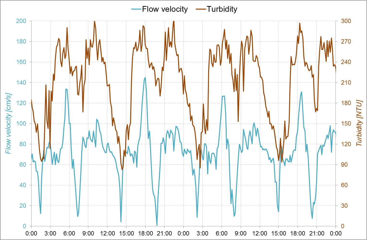
It should be mentioned that this methodology is only a simple approximation of the real sediment fluxes. The methodology uses a constant SPM over the tidal cycle (due to limited data availability), while in reality the SPM will vary strongly over a tidal cycle (Figure 6). Therefore the calculated fluxes should be seen as a first approximation that will be used in the evaluation of topic 3.
Back to top
How can residence times (water/particle) be calculated?
How can sediment transport be managed?
How can we prevent excessive degradation or loss of tidal marshes?
What are the limiting factors of sediment management in the TIDE estuaries regarding hydrogeomorphology?
What factors determine the distribution of suspended sediments in an estuary?
What is important in establishing a zonation for estuaries?
What is the impact of deep subtidal habitat dimension on tidal amplification?
What is the importance of sediment management for integrated estuarine management?
What measures are successful for the dissipation of tidal energy?
Which measures are suitable to achieve specific morphological and hydrological targets?
“Working with nature”: What are the opportunities for sediment management in estuaries?
Interestuarine comparison: Hydro-geomorphology
Table of content
- 1. Introduction
- 1a. Outline
- 2. Objectives
- 3. Methodology
- 3a. Main parameters
- 3b. Derived parameters
- 3c. Habitats
- 3d. Mouth definition
- 4. TIDE estuaries
- 4a. Scheldt
- 4b. Elbe
- 4c. Weser
- 4d. Humber
- 4e. Parameters of the 4 estuaries (TIDE km)
- 5. Interestuarine comparison
- 5a. TOPIC 1 – Tidal amplification
- 5b. TOPIC 2 – Habitats
- 5c. TOPIC 3 – Relation between sediment load and tidal/riverine characteristics
- 5d. TOPIC 4 – Residence time
- 5e. TOPIC 5 – Impact of increasing MHWL on tidal marsh ecosystems
- 6. General conclusions
- 7. References
- 8. Appendix A – Estuary convergence
- 9. Appendix B – Habitat maps
- 10. Appendix C – Habitat widths
- 11. Appendix D – Tidal marsh sites
3b. Derived parameters
Flow velocity, tidal discharge and tidal volume (“Cubage” technique)
IntroductionThe “cubage”-technique (“kubatuur” in Dutch) is a relatively simple technique to calculate the hydrodynamics in an estuary (Smets, 1996; Plancke et aL, 2011). It requires only topo-bathymetric data and water levels at different stations to calculate discharges and cross-sectional averaged flow velocities (see Figure 3) starting from the conservation of mass formula. In contrast to numerical process models, this technique does not require any flow resistance (“roughness”) coefficients to calibrate the model. Where the cubage technique uses mass conservation (which is an exact relationship) the error of the method is solely related to the error in water level and topo-bathymetric data. Hereafter some mathematical background on this technique is given.

The hydrodynamics in a river or estuary can be described in a one-dimensional way using following equations:
- Conservation of mass:
- Dynamic equation:
-
x: abscise of a cross-section in the estuary
z: water level to horizontal reference plain
t: time
Q: discharge, positive from up-estuary to down-estuary (ebb = + | flood = -)
A: area of wet section of cross-section x at water level z: A(x,z)
B: width of a cross-section x at water level z: B(x,z)
u: section-averaged flow velocity: u = Q/A
g: gravitation constant (9,81 m/s²)
C: Chézy roughness coefficient
f: tributary discharge
with:
-
Qn: discharge in cross-section n (up-estuary)
Qn+1: discharge in cross-section n+1 (down-estuary)
Bnt: width of cross-section n at time step t
Dznt,t+1: change in water level for cross-section n, between time step t and t+1
Dx: distance between 2 consecutive cross-sections n en n+1 (500 m)
Dt: time interval between 2 time steps (i.e. temporal resolution of water level measurements; 10 to 15 minutes was chosen in this report)

Output parameters
The “cubage”-technique calculates discharges in time between every 2 consecutive cross-sections in the estuary. From this parameter following additional parameters can be derived:
-
(a) Maximum ebb and flood discharges
(b) Ebb and flood discharges averaged over one tidal cycle

(c) Ebb and flood tidal volumes
(d) Evolution in time of section-averaged velocity

(e) Maximum ebb and flood velocity
(f) Ebb and flood velocities averaged over one tidal cycle
Within the TIDE-project it was chosen to perform the cubage calculation for mean tidal conditions (only input data available for mean tidal conditions). In a first step the mean tidal parameters (HW, LW, time of rising and time of falling) were derived from measurements for the present situation for a station at the mouth, a station in the middle of the estuary, and a station at the upstream boundary of the estuary (see Table 3). Where the cubage technique requires a continuous time series of water levels, one period (or 2 periods for the Elbe and Humber) with several tidal cycles was chosen from the continuous measurements (see ‘selected tides’ Table 3) for which the low and high waters have the best agreement with the MHWL and MLWL values for the present situation for all 3 selected stations. For the Elbe and Humber 2 time periods were selected (one with low and one with high river discharge) because of the important differences in river discharge at the up-estuary boundary of these estuaries. From the selected time period, water level measurements for all tidal stations were selected as input for the cubage calculation (location of all tidal stations see Figure 9 (Scheldt), Figure 10 (Elbe), Figure 11 (Weser) and Figure 12 (Humber)) .
In a next step cross sections were defined perpendicular to the thalweg. The thalweg is defined as the longitudinal profile linking the deepest points of each cross section. The distance between two sections was chosen at about 500 m: this resolution was on the one hand sufficient to represent the topo-bathymetry, while on the other hand the number of cross section remained acceptable. These cross sections were exported in a MIKE11-format. Subsequently the different cross sections were imported in MIKE11 and the necessary parameters for each cross section were derived automatically within this software:
- Wet cross section area at different heights
- Width at different heights
Cubage calculations with a winter/summer condition were within this study performed for 3 of the 4 estuaries (Elbe, Weser and Humber) (see Plancke et al., 2012a,b,c). For the calculation of the high/low discharge period of the Elbe and Humber, appropriate tides were selected in the high/low discharge period with implementation of respectively the P(95%) and P(5%) freshwater discharges. For the Weser, appropriate tides were selected only during one time period of the year. The high/low discharge variation was again simulated by implementation of respectively the P(95%) and P(5%) freshwater discharges. For the Scheldt, an earlier cubage calculation with implementation of a mean freshwater discharge (P(50%)) was used (Plancke et al., 2011). Here, no distinction was thus made between winter and summer condition, due to the limited effect of the discharge on the water level.
More detailed information on the cubage technique is given by Plancke et al. (2012a,b,c).
Table 3 – Input data used for the cubage calculations of each estuary
|
Scheldt | Elbe | Weser | Humber |
Topo-bathymetry |
2001 | 2006 | 2009 | 2005 |
HW and LW |
1991-2000 | 2001-2010 | 2001-2010 | 2005 |
Stations used for selection of mean tide |
Vlissingen Antwerpen Sint-Amands |
Groβer Vogelsand Kollmar Wehr Geesthacht |
LT Alte Weser Nordenham Grosse Weser-brücke |
Spurn Point South Ferriby Naburn Lock (Ouse) Carlton on Trent (Trent) |
Selected tides |
21-22/06/2009 | 5/03/2006 (high Q) 25/05/2006 (low Q) |
7-8/06/2010 | 5-6/01/2005 (high Q) 3-4/05/2005 (low Q) |
Freshwater discharge |
2000-2010 (P50) |
2001-2010 (P95 and P5) |
2001-2010 (P95 and P5) |
2010 (P95 and P5) |
Tidal damping scale
IntroductionThe tidal penetration in an estuary is influenced by several factors, with the most important factors being the funnel shape of the estuary, leading to an amplification of the tidal range, and the friction within the estuary, leading to a decrease in tidal range. The relative importance of these 2 factors is presented in the tidal damping scale (), which is a simple analytical expression to describe tidal amplification or damping (Savenije, 2001). Tidal damping (1/ is defined as:
With:
-
ß = tidal damping scale [m]
b = width convergence length [m]; derived from following regression:
f’ = adjusted friction factor =
v = amplitude of flow velocity (average of maximum ebb and maximum flood velocity at mean tidal
conditions) [m/s]
e = phase lag between HW and slack HW
c = celerity of tidal wave (= sqrt(g.h)) [m/s]
h = averaged water depth over tidal cycle (= (hHW + hLW)/2) [m]
h = tidal amplitude (= tidal range/2) [m]
C = Chézy roughness coefficient [m1/2/s]
g = gravitation constant (9,81 m/s²)
Assumptions
To calculate 1/β the following assumptions were made:
- Data were averaged over 5 km blocks along the thalweg
- Only the estuary was regarded and not the mouth area (based on mouthgeo, for definition see §3.4)
- Data with a ratio TR/h > 0.80 were excluded from the analysis (TR =tidal range, h= averaged water depth over tidal cycle). Above this threshold, tidal damping calculations become less accurate (Savenije, 1998). For the Scheldt, 5 data points were excluded (in total 25 km), for the Humber 11 datapoints (in total 55 km, a consequence of the shallowness of the estuary). For Elbe and Weser no data points were excluded.
- Chézy roughness coefficient C = 50; phase lag difference ε = 50’ (see sensitivity analysis below)
Estuary convergence
In the tidal damping equation (see Equation (1)), the estuary convergence is described by the width convergence length (b). This parameter is determined based on the following equation:
![]()
With:
-
B = the average cross-sectional and tidal-average width (m)
B0 = the width at the estuary mouth (m)
x = the distance from the mouth
Sensitivity analysis
For the Scheldt estuary a sensitivity analysis was performed on the tidal damping scale (Figure 5 ) in relation to the following parameters:
- Chézy roughness coefficient: 40 – 50 – 60
- Phase lag HW – slack HW: 30’ – 50’ – 70’

It was decided to use C = 50 and ε = 50’ to calculate 1/b based on the following criteria:
- There should be a good agreement between 1/b and the change in tidal range: if 1/b > 0 we can expect an increase in tidal range, if 1/b < 0 we can expect a decrease in tidal range
- The selected values for C and ε should be realistic values. A Chézy coefficient of 50 is a commonly used value in estuarine modeling (Savenije, 2001, 2005; van Rijn, 2011; Winterwerp, 2012). However, it should be pointed out that Chézy coefficients may vary in time for one estuary, and in between different estuaries (from 30-80, see Winterwerp (2012)). Under mean tidal conditions, a phase lag difference of 50 minutes is representative for estuaries with semi-diurnal tides (Savenije, 2001)
Table 4 – Overview of the parameters used to calculate 1/b
| Parameter | Scheldt | Elbe | Weser | Humber |
| 1/b [m-1] | 2.42*E-5 (TIDE km 0-52) 3.74*E-5 (TIDE km 52-157) 3.39*E-5 (mean) |
1.16*E-5 (TIDE km 0-24) 3.17*E-5 (TIDE km 24-149) 2.75*E-5 (mean) |
2.79*E-5 | 2.17*E-5 (TIDE km 0-44) 5.4*E-5 (TIDE km 44-114) 4.18*E-5 (mean) |
| v [m/s] | Calculated for each “cubage” cross-section (based on cubage) | |||
| e [minutes] | 50 | 50 | 50 | 50 |
| c [m/s] | Calculated for each “cubage” cross-section | |||
| h [m] | Calculated for each “cubage” cross-section | |||
| h [m] | Calculated for each “cubage” cross-section (based on measured data) | |||
| C [m1/2/s] | 50 | 50 | 50 | 50 |
Sediment fluxes
IntroductionBased on the derived tidal discharges calculated by applying the cubage technique (§3.2.1, see output parameters (b)) and the observed SPM values (see §3.1.4), sediment fluxes can be calculated according to the following equation:
With:
- SF = sediment flux per unit cross section (kg/m²/s)
Cs = concentration suspended particle matter (kg/m³)
Q = tidal discharge over one tidal cycle at mean tidal conditions, positive from up-estuary to down-estuary (ebb = + | flood = -) (m³/s)
A = wet section at mean tidal conditions during half tide (= mean of wet section at low water and high water) (m²)
Tidal discharges over a tidal cycle, representative for mean tidal conditions, were calculated at every water level station (§3.1.2). For the Scheldt these tidal discharges were calculated under conditions of mean riverine discharges (see Plancke et al., 2011). For the Elbe, Weser and Humber tidal discharges were calculated under conditions of high and low riverine discharges (see Plancke et al., 2012a,b,c). If the netto discharge over a tidal cycle is positive than the water is transported in the ebb direction, if the netto discharge over a tidal cycle is negative than the water is transported in the flood direction. SPM values at the water level stations were derived by use of linear interpolation (SPM stations not at the same locations as the water level stations, see Figure 9 till Figure 12). Based on the available SPM data and calculated tidal discharges (see Table 5), sediment fluxes were calculated according to equation (3). The sediment fluxes in the flood direction are hereby positive and the sediment fluxes in the ebb direction are negative (see equation (3)). Sediment fluxes under mean riverine discharges for the Elbe, Weser and Humber were determined by averaging the calculated sediment fluxes under high and low riverine discharge.
For each water level stations a netto sediment flux was calculated, as the sum of the different sediment fluxes per time step over a full tidal cycle.
Table 5 – Overview of the input parameters used to calculate sediment fluxes. (R = riverine discharge)
| SPM | Tidal discharges | |
| Scheldt | surface and watercolumn | mean R |
| Elbe | surface | low and high R |
| Weser | surface | low and high R |
| Humber | surface | low and high R |
It should be mentioned that this methodology is only a simple approximation of the real sediment fluxes. The methodology uses a constant SPM over the tidal cycle (due to limited data availability), while in reality the SPM will vary strongly over a tidal cycle (Figure 6). Therefore the calculated fluxes should be seen as a first approximation that will be used in the evaluation of topic 3.
Important to know
Reports / Measures / Tools
| Report: | Management measures analysis and comparison |
|---|
Management issues
How and by which management measures can tidal amplification be reduced?How can residence times (water/particle) be calculated?
How can sediment transport be managed?
How can we prevent excessive degradation or loss of tidal marshes?
What are the limiting factors of sediment management in the TIDE estuaries regarding hydrogeomorphology?
What factors determine the distribution of suspended sediments in an estuary?
What is important in establishing a zonation for estuaries?
What is the impact of deep subtidal habitat dimension on tidal amplification?
What is the importance of sediment management for integrated estuarine management?
What measures are successful for the dissipation of tidal energy?
Which measures are suitable to achieve specific morphological and hydrological targets?
“Working with nature”: What are the opportunities for sediment management in estuaries?