

Disclaimer:
The authors are solely responsible for the content of this report. Material included herein does not represent the opinion of the European Community, and the European Community is not responsible for any use that might be made of it.
Back to overview reports
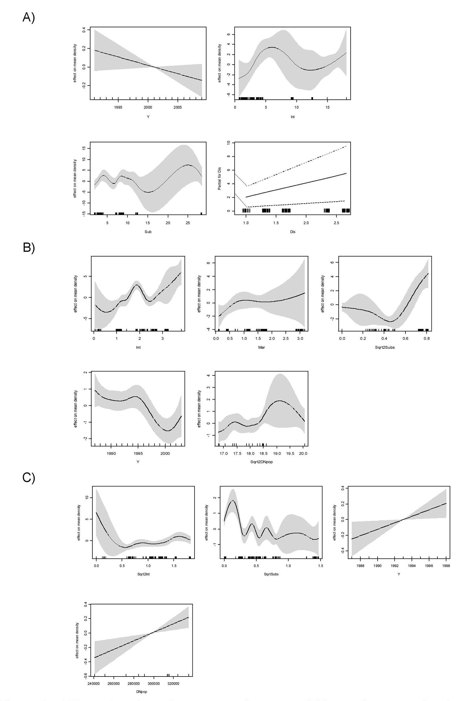
The best models, as selected by the analysis, included 4 to 5 variables, which explained more than 75% of the total variability in the species density distribution in the estuaries (Table 5, Figure 6). All these models include intertidal and subtidal habitat (shallow subtidal in particular in the Weser and Elbe models) among the predictors, these two variables ranking between first and fourth in terms of their importance in affecting the species density distribution (as single predictor models). Marsh area is included as an additional habitat variable in the Weser model (scoring 2 in terms of ranked importance as a single predictor), although its effect on Dunlin density in the other estuaries cannot be ruled out, due to its positive correlation with the intertidal area in them. In both the Humber and the Weser, a general increase of mean density of Dunlin is predicted where larger habitat areas occur, although the range of variability of these covariates is markedly different between the two estuaries, due to the larger area of sectors in the Humber (between 6 and 42 km2, 17 km2 on average) compared to the area of the counting units in the Weser (between 0.4 and 21 km2, 5 km2 on average)¹ (Figure 6). Besides these differences, a general low density of Dunlin is expected when the intertidal area in the sector/unit is <1 km2, whereas higher density is predicted to be found with intertidal areas >3 km2 in the Weser and >16 km2 in the Humber (although relative higher density is predicted also with intertidal area between 3 and 9 km2 in this latter estuary). An increase in Dunlin density is also predicted with higher subtidal area (>0.9 km2 in the Weser, and >20 km2 in the Humber, with a maximum at around 25 km2) and with increasing marsh area (in particular with values >2.5 km2) in the Weser, although a similar relationship can be expected also in the Humber, given the positive correlation of marsh area with the intertidal area in the sectors. The results obtained for the Elbe estuary show an opposite relationship of Dunlin density with the habitat areas (in particular intertidal and shallow subtidal), with higher density values expected at smaller habitat areas (<0.8 km2 intertidal, <0.7 km2 shallow subtidal). It is of note also that, when the effect of habitat area is excluded, the relationship with the salinity gradient is still relevant to Dunlin density in the Elbe estuary (with salinity zone included in the final model) with higher Dunlin density expected in oligohaline and mesohaline zones.
Predictors such as year and population size are also selected as relevant to the species density distribution (these two variables being negatively correlated in the Humber), indicating that the density of Dunlin observed in the estuarine habitats may be significantly affected by inter-annual local fluctuations as well as by the temporal changes of the population size at a wider spatial (regional/national) scale. However, it is of note that this temporal variability is of lower importance compared to the effect of spatial (habitat) variables on Dunlin density, confirming the general results derived for the whole bird assemblage (as obtained from the multivariate analysis). The disturbance index was also identified as a relevant predictor of Dunlin density in the Humber Estuary. Contrary to what would be expected, higher density values were predicted in sectors with higher values of the disturbance index (NF, NG and NK, in particular; Appendix 1). This is likely to be an artefact of the analysis derived from the possible inadequacy of the measured index as a proxy for disturbance in the present analysis, rather than being a reflection of a real preference of the species for more disturbed areas (see Discussion for a detailed explanation).
¹ The habitat area in fact is calculated using single sectors/counting units as spatial units, therefore the maximum habitat area measured has the area of the sector/counting unit as upper limit.
When the probability of occurrence of Dunlin is modelled in the Elbe estuary, in relation to either habitat data or water quality variables, it is evident that a lower proportion (<45%) of the data variability is explained by the selected models compared to the density models (>75%), with a higher percentage of deviance explained by the habitat dataset compared to the water quality one (Table 5).
Both models include salinity as a relevant predictor, this variable being among the first two variables in order of importance for their influence on the species distribution, with a higher probability of Dunlin occurrence at intermediate salinities (chlorinity values between 1 and 2.5 mmol/l), in oligohaline and mesohaline zones, when the effect of habitat area is excluded (Figure 7). In the habitat model, shallow subtidal area is again identified as a relevant predictor of Dunlin distribution, although a clear pattern is not evident from the shape of this effect (Figure 7). Also marsh area (Foreland) is included as a relevant predictor in the model, being the most important one among those considered. A higher probability of occurrence for the species is expected with lower marsh area (<0.9 km2), a condition that is also usually associated with lower intertidal area (as these two variables are positively correlated in the Elbe). This negative relationship of Dunlin occurrence with the marsh and intertidal habitat area is likely to be an artefact of the analysis rather than reflecting a real preference of the species for smaller marsh and intertidal areas. In fact, the analysed dataset for the Elbe included very small counting units (hence leading to small habitat areas in them) where Dunlin was detected with very high frequency and numbers, an effect that is likely to be the consequence of the location of these units in undisturbed and remote zones within the extensive mudflat areas available in the Waddensea.
As regards the water quality model, both nutrients concentrations (as PO4 and autumn NH4) are included as relevant predictors of the species occurrence, with lower probability of presence in areas where PO4 is higher and NH4 is between 0.003 and 0.006 mmol/l (Figure 7). ). In both models, the location of the counting unit with respect to the north and south bank of the estuary (with higher probability of presence in the north bank than in the south bank) and the year are also selected as relevant to the species distribution, although these variables have a lower importance (scoring 5 to 7 in terms of ranked importance as a single predictor) compared to the others included in the models.
Back to top
What environmental factors should be considered in the design of a compensation scheme for waterbirds and their habitats?
What environmental variables are most important in determining minimizing or basic compensatory requirements for waterbirds?
What is important in establishing a zonation for estuaries?
What tools and guidance are available to minimise and mitigate disturbance to waterbirds?
Determinants of bird habitat use in TIDE estuaries
Table of content
- 1. SUMMARY
- 2. INTRODUCTION
- 3. STRUCTURE OF THE REPORT
- 4. DATA USED
- 5. GENERAL CHARACTERISTICS OF BIRD ASSEMBLAGES IN TIDE ESTUARIES
- 6. BIRD ASSEMBLAGES DISTRIBUTION AND RELATIONSHIP WITH ENVIRONMENTAL VARIABLES
- 6a. Humber
- 6b. Weser
- 6c. Elbe
- 7. SPECIES DISTRIBUTION MODELS
- 7a. Dunlin
- 7b. Redshank, Golden Plover and Bar-tailed Godwit
- 7c. Shelduck, Pochard and Brent Goose
- 8. DISCUSSION
- 9. CONCLUSIONS
- 9a. Analysis Conclusions
- 9b. Management Recommendations
- 9c. Recommendations for Future Studies
- 10. REFERENCES
- 11. APPENDIX 1
- 12. APPENDIX 2
- 13. APPENDIX 3
- 14. APPENDIX 4
7a. Dunlin
Dunlin distribution was analysed in all the three estuaries and, in most of cases, the species mean density was modelled (Appendix 4). Only in the Elbe the density of the species could not be related to water quality variables, therefore the probability of occurrence was modelled instead. A summary of the resulting models obtained for Dunlin in the studied estuaries is reported in Table 5 and the shape of the effect of each selected continuous predictor variable on the model response is shown in Figure 6 and Figure 7.The best models, as selected by the analysis, included 4 to 5 variables, which explained more than 75% of the total variability in the species density distribution in the estuaries (Table 5, Figure 6). All these models include intertidal and subtidal habitat (shallow subtidal in particular in the Weser and Elbe models) among the predictors, these two variables ranking between first and fourth in terms of their importance in affecting the species density distribution (as single predictor models). Marsh area is included as an additional habitat variable in the Weser model (scoring 2 in terms of ranked importance as a single predictor), although its effect on Dunlin density in the other estuaries cannot be ruled out, due to its positive correlation with the intertidal area in them. In both the Humber and the Weser, a general increase of mean density of Dunlin is predicted where larger habitat areas occur, although the range of variability of these covariates is markedly different between the two estuaries, due to the larger area of sectors in the Humber (between 6 and 42 km2, 17 km2 on average) compared to the area of the counting units in the Weser (between 0.4 and 21 km2, 5 km2 on average)¹ (Figure 6). Besides these differences, a general low density of Dunlin is expected when the intertidal area in the sector/unit is <1 km2, whereas higher density is predicted to be found with intertidal areas >3 km2 in the Weser and >16 km2 in the Humber (although relative higher density is predicted also with intertidal area between 3 and 9 km2 in this latter estuary). An increase in Dunlin density is also predicted with higher subtidal area (>0.9 km2 in the Weser, and >20 km2 in the Humber, with a maximum at around 25 km2) and with increasing marsh area (in particular with values >2.5 km2) in the Weser, although a similar relationship can be expected also in the Humber, given the positive correlation of marsh area with the intertidal area in the sectors. The results obtained for the Elbe estuary show an opposite relationship of Dunlin density with the habitat areas (in particular intertidal and shallow subtidal), with higher density values expected at smaller habitat areas (<0.8 km2 intertidal, <0.7 km2 shallow subtidal). It is of note also that, when the effect of habitat area is excluded, the relationship with the salinity gradient is still relevant to Dunlin density in the Elbe estuary (with salinity zone included in the final model) with higher Dunlin density expected in oligohaline and mesohaline zones.
Predictors such as year and population size are also selected as relevant to the species density distribution (these two variables being negatively correlated in the Humber), indicating that the density of Dunlin observed in the estuarine habitats may be significantly affected by inter-annual local fluctuations as well as by the temporal changes of the population size at a wider spatial (regional/national) scale. However, it is of note that this temporal variability is of lower importance compared to the effect of spatial (habitat) variables on Dunlin density, confirming the general results derived for the whole bird assemblage (as obtained from the multivariate analysis). The disturbance index was also identified as a relevant predictor of Dunlin density in the Humber Estuary. Contrary to what would be expected, higher density values were predicted in sectors with higher values of the disturbance index (NF, NG and NK, in particular; Appendix 1). This is likely to be an artefact of the analysis derived from the possible inadequacy of the measured index as a proxy for disturbance in the present analysis, rather than being a reflection of a real preference of the species for more disturbed areas (see Discussion for a detailed explanation).
¹ The habitat area in fact is calculated using single sectors/counting units as spatial units, therefore the maximum habitat area measured has the area of the sector/counting unit as upper limit.

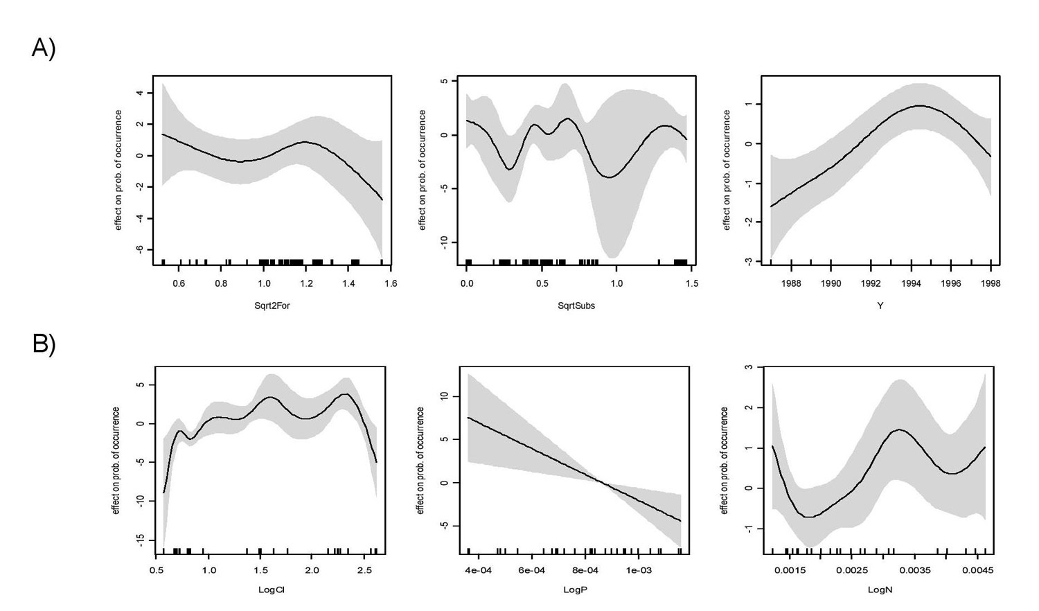
When the probability of occurrence of Dunlin is modelled in the Elbe estuary, in relation to either habitat data or water quality variables, it is evident that a lower proportion (<45%) of the data variability is explained by the selected models compared to the density models (>75%), with a higher percentage of deviance explained by the habitat dataset compared to the water quality one (Table 5).
Both models include salinity as a relevant predictor, this variable being among the first two variables in order of importance for their influence on the species distribution, with a higher probability of Dunlin occurrence at intermediate salinities (chlorinity values between 1 and 2.5 mmol/l), in oligohaline and mesohaline zones, when the effect of habitat area is excluded (Figure 7). In the habitat model, shallow subtidal area is again identified as a relevant predictor of Dunlin distribution, although a clear pattern is not evident from the shape of this effect (Figure 7). Also marsh area (Foreland) is included as a relevant predictor in the model, being the most important one among those considered. A higher probability of occurrence for the species is expected with lower marsh area (<0.9 km2), a condition that is also usually associated with lower intertidal area (as these two variables are positively correlated in the Elbe). This negative relationship of Dunlin occurrence with the marsh and intertidal habitat area is likely to be an artefact of the analysis rather than reflecting a real preference of the species for smaller marsh and intertidal areas. In fact, the analysed dataset for the Elbe included very small counting units (hence leading to small habitat areas in them) where Dunlin was detected with very high frequency and numbers, an effect that is likely to be the consequence of the location of these units in undisturbed and remote zones within the extensive mudflat areas available in the Waddensea.
As regards the water quality model, both nutrients concentrations (as PO4 and autumn NH4) are included as relevant predictors of the species occurrence, with lower probability of presence in areas where PO4 is higher and NH4 is between 0.003 and 0.006 mmol/l (Figure 7). ). In both models, the location of the counting unit with respect to the north and south bank of the estuary (with higher probability of presence in the north bank than in the south bank) and the year are also selected as relevant to the species distribution, although these variables have a lower importance (scoring 5 to 7 in terms of ranked importance as a single predictor) compared to the others included in the models.
Important to know
Reports / Measures / Tools
| Report: | Management measures analysis and comparison |
|---|
Management issues
How can management targets and monitoring strategies be set for waterbirds in compensatory areas?What environmental factors should be considered in the design of a compensation scheme for waterbirds and their habitats?
What environmental variables are most important in determining minimizing or basic compensatory requirements for waterbirds?
What is important in establishing a zonation for estuaries?
What tools and guidance are available to minimise and mitigate disturbance to waterbirds?